万能的qplot——更精致的展现
之前的文章已经为大家介绍过了万能的qplot——基础,这次给大家说一说qplot的精致展现。
一、组合geoms和stats
d <- ggplot(diamonds, aes(carat)) + xlim(0, 3)
d + stat_bin(aes(ymax = ..count..), binwidth = 0.1, geom = "area")
d + stat_bin(
aes(size = ..density..), binwidth = 0.1,geom = "point", position="identity")
d + stat_bin(
aes(y = 1, fill = ..count..), binwidth = 0.1,geom = "tile", position="identity")

二、基本作图类型
1.线图
p + geom_line() + ggtitle( "geom_line")

2.填充图
p + geom_area() + ggtitle("geom_area")

3.路径图
p + geom_path() + ggtitle("geom_path")

三、通过散点形状和大小控制重叠
df <- data.frame(x = rnorm(2000), y = rnorm(2000))
norm <- ggplot(df, aes(x, y))
norm + geom_point()
norm + geom_point(shape = 1)
norm + geom_point(shape = ".") # Pixel sized

四、扰动(jitter)表示法
jit <- position_jitter(width = 0.5)
td + geom_jitter(position = jit)
td + geom_jitter(position = jit, colour = alpha("black", 1/10))
td + geom_jitter(position = jit, colour = alpha("black", 1/50))
td + geom_jitter(position = jit, colour = alpha("black", 1/200))
表示法.png")
关于万能的qplot——更精致的展现的讲述就到这里了,上述的内容只是截取了资料中的一部分,如需获取完整的资料,可通过关注微信公众号后联系客服获取。
想要了解更多的资料、信息,可持续关注我们,我们将为大家提供有价值、有需求的材料。为大家在整理数据时省去烦恼。
 打开微信“扫一扫”,打开网页后点击屏幕右上角分享按钮

-
论文打印要求是什么,单面还是双面? 132138
-
 ieee论文什么水平,含金量如何? 71408
-
大肠杆菌转化实验技术分享 2019.06.24 15:38
-
我做医学科研的体会 2019.06.24 14:59
-
SCI英文写作中常用句型汇总 2019.06.24 11:13
-
医学研究生的科研开题报告怎么写 2019.06.21 16:17
-
 单变量方差分析之spss实现步骤
 -
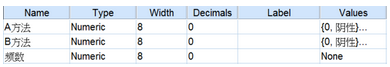
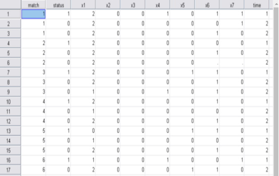 如何用SPSS处理1:N匹配的病例对照研究资料
 -
 配对卡方检验与一致性检验的SPSS操作步骤
